Why Single Strategies Eventually Fail
Every trading strategy captures a specific market effect: mean reversion, momentum, volatility expansion, seasonal patterns, or structural inefficiencies. These effects exist because of human behavior, institutional flows, or market microstructure — and they’re real.
But no single effect persists in every market regime.
A mean-reversion strategy thrives in range-bound, choppy markets. Put it in a trending market and it gets slaughtered — repeatedly buying dips that keep dipping. A momentum strategy does the opposite: it crushes trending markets but gets whipsawed in sideways chop. A volatility-selling strategy prints money in calm markets and blows up in a crisis.
This isn’t a flaw in the strategies. It’s a feature of markets. Regimes change. Volatility expands and contracts. Trends emerge and mean-revert. No single strategy can adapt to all of these shifts simultaneously — and adding more rules to make it “adaptive” just creates a more complex, more overfit system.
The Math: Why Portfolios Work
The concept is intuitive: when one strategy is losing, another should be winning (or at least flat). But the math behind why this works is more powerful than most traders realize.
Drawdown Compression
Consider three strategies that each have a 40% maximum drawdown at some point in their history. Sounds terrible for each one individually. But if those drawdowns don’t happen at the same time — because the strategies are trading different effects across different markets — the combined portfolio might never exceed a 5% drawdown.
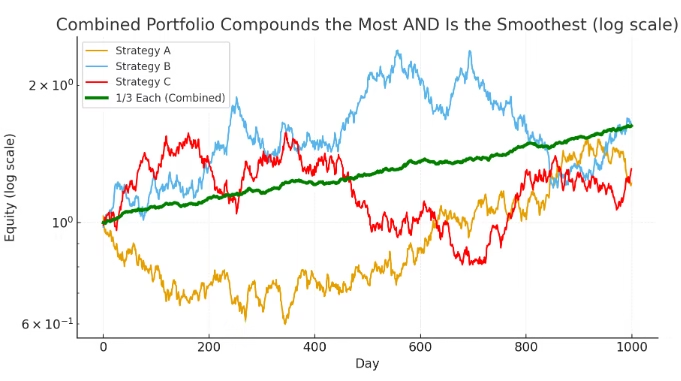
Three individually mediocre strategies combine into a portfolio with dramatically better risk-adjusted returns.
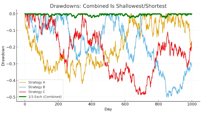
Each strategy experienced a 40%+ drawdown individually — the combined portfolio never exceeded 5%.
The key requirement: low correlation between the strategies. If all three strategies lose at the same time, the portfolio offers no benefit. But if they take turns leading and lagging — like pistons in a car engine — the ride smooths out dramatically.
Shannon’s Demon and the Rebalancing Premium
There’s an even more surprising result. Under certain conditions, you can combine two losing strategies into a winning portfolio. This echoes Parrondo’s Paradox in game theory — the idea that combining losing games can produce a winning game.
The mechanism is rebalancing. When you periodically reset your capital allocation back to target weights — say 50/50 — you mechanically sell what just went up and buy what just went down. When strategies are sufficiently uncorrelated and volatile, this creates a rebalancing premium.
The math: geometric return is approximately the arithmetic return minus half the variance. When you combine uncorrelated strategies and rebalance, the portfolio variance drops much faster than the arithmetic mean. This can flip a negative geometric return positive — turning a losing portfolio into a winning one, purely from the discipline of rebalancing.
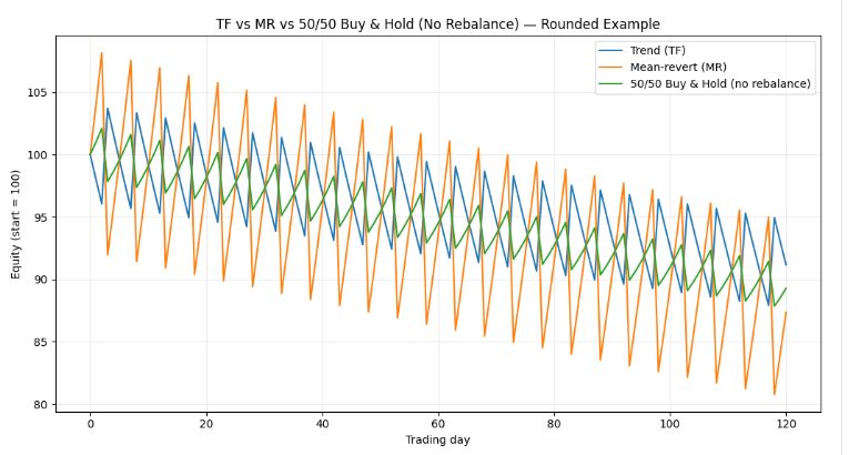
Without rebalancing: two individually losing strategies combined still lose (green line).
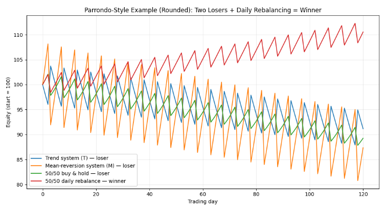
With daily rebalancing (red): the same two losers become a winner. This is Shannon’s Demon in action.
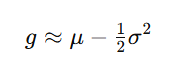
The formula behind the rebalancing premium: as portfolio variance drops, geometric return rises.
But this isn’t magic. It only works when strategies have low or negative correlation and enough volatility to provide a harvestable dispersion premium. If strategies are highly correlated, rebalancing does nothing useful. And transaction costs can erase the premium if you rebalance too frequently. This is why proper portfolio backtesting — with shared capital, realistic costs, and configurable rebalancing — matters so much.
How Sharpe Ratio Scales With More Strategies
Here’s the result that should permanently change how you allocate your research time.
For a portfolio of n strategies with equal Sharpe ratios (S) and equal pairwise correlation (ρ), the portfolio Sharpe ratio is approximately:
When strategies are perfectly uncorrelated (ρ = 0), this simplifies beautifully: the portfolio Sharpe scales with the square root of n. Two uncorrelated strategies with individual Sharpe ratios of 0.5 produce a portfolio Sharpe of roughly 0.71. Four produce 1.0. Nine produce 1.5. Sixteen produce 2.0.
To put real numbers to this:
| Strategies (n) | Individual Sharpe | Portfolio Sharpe (ρ=0) | Improvement |
|---|---|---|---|
| 1 | 0.50 | 0.50 | — |
| 2 | 0.50 | 0.71 | +41% |
| 4 | 0.50 | 1.00 | +100% |
| 9 | 0.50 | 1.50 | +200% |
| 16 | 0.50 | 2.00 | +300% |
This is extraordinary. Four mediocre strategies — each with a Sharpe of 0.50 that you’d barely consider trading alone — combine into a portfolio with a Sharpe of 1.0, which is institutional quality. You didn’t improve any individual strategy. You just combined them.
Of course, the ρ = 0 assumption is the ideal case. In practice, strategies are rarely perfectly uncorrelated. But even with moderate positive correlation (say ρ = 0.2), the scaling effect remains powerful — it just flattens earlier. The table below shows the difference:
| Strategies (n) | Portfolio Sharpe (ρ=0) | Portfolio Sharpe (ρ=0.2) | Portfolio Sharpe (ρ=0.5) |
|---|---|---|---|
| 1 | 0.50 | 0.50 | 0.50 |
| 4 | 1.00 | 0.76 | 0.63 |
| 9 | 1.50 | 0.96 | 0.70 |
| 16 | 2.00 | 1.10 | 0.75 |
| ∞ | ∞ | 1.12 | 0.71 |
At high correlation (ρ = 0.5), adding strategies beyond 4 or 5 barely helps — you’re just taking the same bet multiple times. But at ρ = 0.2 (achievable with genuine style, asset, and timeframe diversification), you can roughly double a 0.50 Sharpe with 16 strategies. And at ρ = 0? The sky is the limit, mathematically.
The practical takeaway: one hour spent finding a new uncorrelated strategy is worth more than ten hours spent improving an existing one. The Sharpe improvement from combining is structural. The Sharpe improvement from tweaking parameters is fragile and often overfit.
Build Alpha’s Portfolio Suggest AI automates this process — sifting through your saved strategies to find the combinations, weightings, and sizing methods that maximize risk-adjusted returns. The blue lines below are various portfolio combinations Build Alpha simulated; the red line is buy and hold.
Portfolio Suggest AI: one button generates optimal strategy combinations, weightings, and sizing methods.
How Professional Traders Build Strategy Portfolios
The quant funds I’ve consulted for don’t deploy one strategy. They deploy dozens or hundreds, diversified across multiple dimensions:
- Asset class diversification — equities, futures, forex, commodities, bonds. Different asset classes are driven by different fundamental forces, which naturally produces low correlation between strategies.
- Timeframe diversification — intraday, daily, weekly. A strategy that trades every few hours and a strategy that holds for weeks rarely experience drawdowns simultaneously.
- Style diversification — mean reversion, momentum, trend following, volatility, market making. These are fundamentally different approaches to extracting edge, and they tend to perform in opposite market conditions.
- Signal diversification — price action, volume, volatility indicators, sentiment, fundamentals, intermarket signals. Different inputs create different behaviors even within the same style.
The goal isn’t just “more strategies.” It’s uncorrelated strategies that cover different market environments. Five momentum strategies on the S&P 500 is not a portfolio — it’s the same bet five times. One momentum strategy on equities, one mean-reversion strategy on bonds, one volatility strategy on commodities, and one seasonal strategy on currencies? That’s a portfolio.
The Strategy Styles That Matter
When I talk about diversifying across “styles,” traders sometimes nod along but aren’t sure what the categories actually are. Here are the major strategy styles — or market effects — that professional portfolio builders use. Each exploits a different structural reason why prices move, which is precisely why they tend to be uncorrelated with each other.
Trend Following / Momentum
The oldest and most documented systematic style. Trend following profits when markets move directionally — up or down — for extended periods. It suffers in choppy, range-bound conditions where false breakouts accumulate. The classic profile: low win rate (30–40%) offset by very large winners. Trend followers often use moving average crossovers, breakout signals, or channel systems.
When it works: trending markets, crises (often on the short side), macro regime shifts.
When it struggles: sideways chop, mean-reverting periods, whipsaws.
Mean Reversion
The natural counterpart to momentum. Mean-reversion strategies profit when prices overshoot and snap back — buying dips in uptrends, selling rips in downtrends. They tend to have high win rates (65–85%) with smaller average wins and the occasional large loss when the “reversion” never comes and a dip becomes a crash.
When it works: range-bound markets, high-volatility chop, post-overreaction snaps.
When it struggles: strong trends, market crashes (catching falling knives).
Carry
Carry strategies earn the yield differential between instruments or asset classes. In currencies, this means going long high-yielding currencies and short low-yielding ones. In futures, it means harvesting the roll yield from contango or backwardation. In equities, dividend-capture strategies are a form of carry. The returns are typically steady and small, punctuated by sharp reversals during risk-off events.
When it works: calm, risk-on environments with stable interest rate differentials.
When it struggles: sudden risk-off events, carry unwinds, central bank surprises.
Volatility
Strategies that trade the level or structure of volatility itself. Short-volatility strategies (selling options, selling VIX) earn a steady premium in calm markets but face catastrophic risk in spikes. Long-volatility strategies (buying options, tail risk hedging) bleed slowly but produce large gains during crises. Relative-value volatility strategies trade the term structure or skew.
When it works: depends heavily on direction — short vol thrives in calm, long vol thrives in chaos.
When it struggles: the opposite regime of whichever direction you’re exposed to.
Seasonal / Calendar
Strategies based on recurring calendar patterns: end-of-month flows, holiday effects, turn-of-month patterns, day-of-week tendencies, or quarterly rebalancing windows. These effects are often driven by institutional behavior (pension fund flows, index rebalances, options expiration) rather than price patterns, which makes them fundamentally different from technical strategies.
When it works: when institutional flows dominate price action.
When it struggles: when macro events override typical calendar behavior.
Event-Driven / News
Strategies that trade around specific catalysts: earnings announcements, economic data releases (FOMC, NFP, CPI), geopolitical events, or corporate actions. The edge comes from positioning before, during, or after the event — often exploiting the predictable volatility pattern that surrounds scheduled releases. Build Alpha includes historical economic news and event data for exactly this purpose.
When it works: around scheduled events with predictable market reactions.
When it struggles: when event outcomes surprise consensus, or when events are priced in.
Why This Taxonomy Matters for Portfolios
The reason to understand these categories isn’t academic — it’s practical. Each style tends to make money in market conditions where the others lose. Trend following and mean reversion are near-opposites. Carry and volatility selling both bleed during crises while long-volatility strategies and trend followers profit. Seasonal strategies often have low correlation to everything because they’re driven by calendar mechanics rather than price behavior.
A well-constructed portfolio includes strategies from at least 3–4 of these categories across multiple asset classes. That’s how you get the low correlation that drives the Sharpe scaling and drawdown compression described above. Build Alpha’s correlation matrix makes it easy to verify that the strategies you’re combining are actually capturing different effects rather than making the same bet in different wrappers.
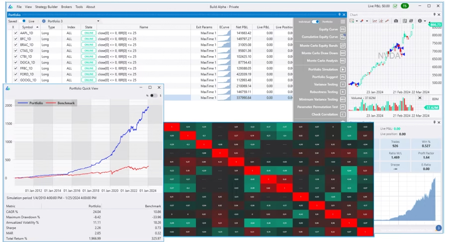
Build Alpha’s portfolio analysis: equity curve vs. buy and hold, correlation matrix, and per-strategy risk metrics — all in one view.
The Pitfall Most Traders Don’t See
Most “portfolio backtesting” tools merge trade lists from separately backtested strategies. Strategy A produced these trades. Strategy B produced those trades. Stack them together. Done.
This is wrong.
When strategies share capital, the results change. A strategy that sizes positions based on stop-loss distance might take 3 trades in isolation because capital was fully deployed. In a real portfolio, profits from other strategies free up capital for a 4th trade — one that never appeared in the standalone backtest.
True portfolio simulation requires re-running all strategies simultaneously with shared capital, tracking how capital flows between strategies in real time, and modeling position sizing as it would actually work with a shared account balance.
This is why I built Build Alpha’s Portfolio Mode to re-simulate rather than merge — the results can differ significantly. It’s built for both independent traders and professional managers (CTAs and RIAs) running multiple strategies across multiple client accounts.
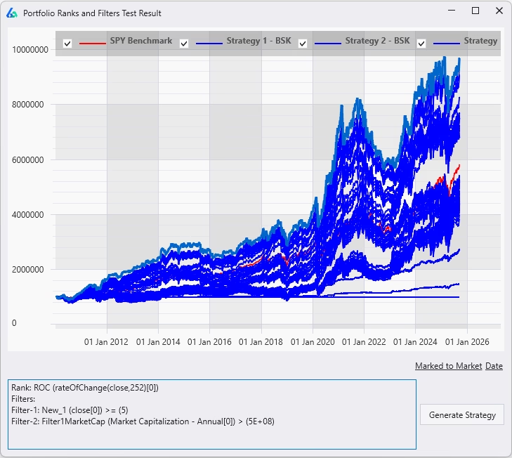
Build Alpha tests different filter and ranking combinations to find the best configuration for your portfolio — not just the strategy.
Building Your Own Strategy Portfolio
If you’re currently trading one system, or researching strategies one at a time, here’s a practical framework for transitioning to portfolio thinking:
Start with what you have. If you have one profitable, robust strategy, don’t abandon it. Ask: what market conditions does it struggle in? Then build or find a strategy that thrives in those conditions.
Measure correlation, not just performance. A strategy with mediocre standalone metrics might be the most valuable addition to your portfolio if it’s negatively correlated with everything else you trade. Build Alpha provides a correlation matrix at the portfolio level for exactly this purpose.
Diversify across dimensions. Don’t just add more strategies on the same market and timeframe. Cross different asset classes, holding periods, and strategy styles.
Test the portfolio, not just the pieces. Run Monte Carlo simulations at the portfolio level. Run the noise test on the portfolio. A portfolio that passes robustness testing is far more trustworthy than one built from individually-tested components that were never validated together.
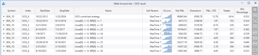
Walk Forward testing at the portfolio level — each row is an out-of-sample period, expandable to show per-strategy performance.
Use proper portfolio backtesting software. Tools that merge trade lists are a starting point, but they can’t model shared capital correctly. You need a capital-aware portfolio simulator that re-runs strategies with shared capital allocation.
Monitor with a daily position report. Build Alpha runs an overnight update on every saved strategy — entries, exits, current positions, rankings, open P&L, funds available, and total exposure — so you know exactly what to do before the market opens.
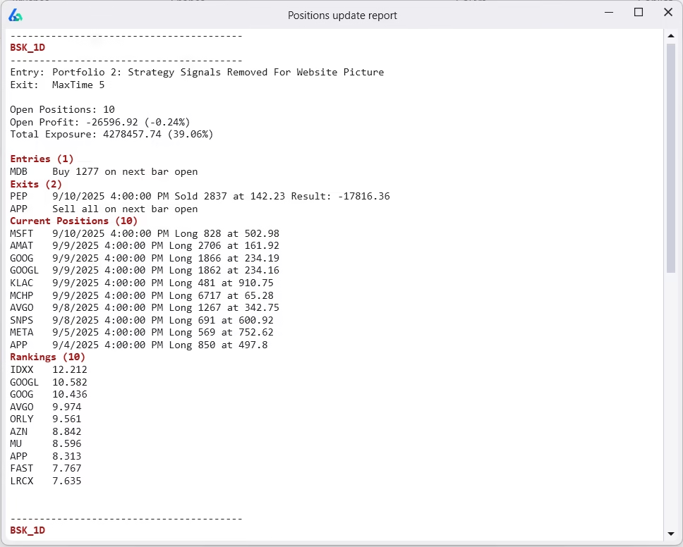
Daily Position Update Report: entries, exits, rankings, P&L, and exposure — updated overnight, ready before the open.
The Bottom Line
The best traders in the world don’t trade one strategy. They trade portfolios. They’ve learned — through painful experience and rigorous math — that no single strategy survives all market regimes, that combining uncorrelated strategies compresses drawdowns in ways that no individual strategy can match, and that the discipline of rebalancing can create returns from volatility itself.
If you’re spending all your research time trying to find one perfect system, you’re solving the wrong problem. The real edge isn’t in the strategy. It’s in the portfolio.
To see how this works in practice — including Parrondo’s Paradox examples, Shannon’s Demon demonstrations, and a walkthrough of every portfolio feature — read the complete Portfolio Backtesting & Trading Guide.
And if you want to see what it looks like to go from lying backtests to validated, portfolio-ready strategies, walk through the Lying Backtests Case Study.